Treating Time as a First-Class Citizen: 4D Gaussian Splatting vs. Deformable 3D Gaussians for Dynamic Scenes

Two modern paths for photorealistic dynamic view synthesis are emerging. One treats spacetime as a single 4D volume (4DGS) and learns 4D primitives with time-evolving appearance. The other keeps 3D Gaussians in a canonical space and learns a deformation field over time (Deformable-GS). This post dissects both, down to implementable equations and training schedules, with a focus on monocular setups.

Introduction

Dynamic scene reconstruction asks us to synthesize novel views of scenes that change over time. It is tougher than the static case for two primary reasons:

1. Motion ambiguity. Occlusions, disocclusions, and non-rigid deformations break multi-view consistency.
2. Temporal coherence. Per-frame reconstructions stitched afterwards waste cross-time signal and often flicker.

Historically, two families dominated: (i) frame-wise models later fused into a dynamic scene; (ii) canonical-space models that explain dynamics as motion or deformation of a single underlying representation. Both can struggle to preserve correlations across distant spacetime locations without interference in messy real-world footage.

This article focuses on two state-of-the-art directions that push beyond these limitations:

• 4D Gaussian Splatting (4DGS). It makes time first-class by optimizing a set of 4D Gaussian primitives with explicit geometry and time-evolving, view-dependent appearance modeled via a combined SH × Fourier basis (a 4D spherindrical harmonic expansion). A splatting renderer then produces photo-real video at well beyond real-time.
• Deformable 3D Gaussians (Deformable-GS). It learns time-independent 3D Gaussians in a canonical space and a deformation MLP that outputs per-time offsets to position, rotation, and scale, plus an Annealing Smoothing Training (AST) schedule that stabilizes monocular videos.

Roadmap. We recap 3DGS [1], then detail 4DGS (primitives, 4D rotations, conditional and marginal math, temporal appearance, rendering, training), then Deformable-GS (canonical modeling, deformation MLP, AST, pitfalls). We end with a practical “which to use when” guide and copy-ready notes.

1. Primer: 3D Gaussian Splatting (3DGS)

3DGS represents a scene as anisotropic 3D Gaussians with opacity $\alpha$ and view-dependent color modeled by spherical harmonics (SH). Each Gaussian is projected to a screen-space elliptical footprint and composited front-to-back with correct depth ordering. The key ingredients:

• Primitives. Centers $\mu\in\mathbb{R}^3$, covariance $\Sigma\in\mathbb{R}^{3\times3}$ factored via rotation quaternion $r$ and scale $s$.
• Projection. Around a mean point, the 2D covariance is approximated by the Jacobian of the camera projection $J$: $\Sigma' \approx J\, \Sigma\, J^\top + \epsilon I$. Standard 3DGS implementations use this or an equivalent closed form.
• Alpha compositing. With per-pixel 2D density $\rho_i(u,v)$ and opacity $\alpha_i$, weight $w_i = \alpha_i\, \rho_i$. Rendering uses front-to-back transmittance $T_{i-1}=\prod_{j<i}(1-w_j)$ and color basis $c_i(\mathbf{d})=\sum_{l,m} a^{(i)}_{lm} Y^m_l(\theta,\phi)$:

Keep this mental model: primitives + SH + splatting + densification. Both 4DGS and Deformable-GS extend it to time.

2. 4D Gaussian Splatting (4DGS) [2]

2.1. 4D primitives and rotations

A 4D Gaussian $\mathcal{N}(\mu\in\mathbb{R}^4, \Sigma\in\mathbb{R}^{4\times4})$ models spacetime directly with coordinates $(x,y,z,t)$. The covariance encodes anisotropy and orientation across space and time. In 4D, any proper rotation decomposes into a pair of plane rotations; in practice, parameterization can leverage two quaternions or an equivalent minimal representation to orient ellipsoids in $(x,y,z,t)$. This lets a primitive tilt through time, aligning with motion trajectories.

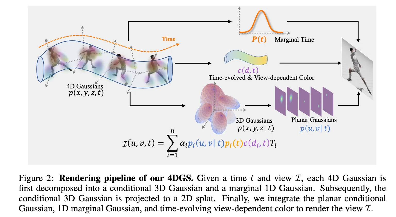
2.2. Correct conditional and marginal factorization

Let the joint variable be $[\mathbf{x}; t]$ with mean $\mu=[\mu_x;\,\mu_t]$ and covariance partitioned as

Then the conditional 3D Gaussian at time $t$ is

with temporal marginal $t\sim\mathcal{N}(\mu_t,\,\Sigma_{tt})$. These block-Gaussian identities are the core of 4DGS’s slice then render view: at any timestamp, each 4D primitive induces a 3D Gaussian.

Trajectory intuition. The curve $\mu_{x\mid t}$ traces a spatial path for each primitive as time varies; 4D rotation plus cross-covariance $\Sigma_{xt}$ lets this path align with intrinsic motion without explicit supervision.

2.3. Rendering and compositing at time $t$

For a camera with intrinsics $K$ and extrinsics $E$, we:

1. Slice. Convert each 4D primitive to its conditional 3D Gaussian at timestamp $t$ using the formulas above.
2. Project. Compute the screen-space footprint $\rho_i(u,v\mid t)$ from $\Sigma_{x\mid t}$ using the projection Jacobian.
3. Gate by time. Use the temporal marginal $\pi_i(t)$ to softly gate visibility.
4. Composite. Define the per-pixel weight

and render

This unified rendering respects both spatial ordering and the likelihood that a primitive is active at time $t$.

2.4. Time-evolving, view-dependent appearance with a 4D basis

Naively storing a separate SH vector per time duplicates coefficients and couples appearance across timestamps. 4DGS instead expands appearance in a tensor-product basis: 3D SH for view dependence and a Fourier series for time:

A small number of temporal modes is typically sufficient. In practice, normalize time to $[0,T)$ per clip and share the Fourier period with the clip length.

2.5. Training, densification, and stability

Sampling across time. Batch timestamps uniformly or proportionally to frame count to reduce flicker and encourage smooth appearance.

Densification and pruning. Track the usual 3DGS signals such as gradient norms and screen-space coverage. For 4DGS add the average gradient of $\mu_t$ as an extra density indicator. Rapid temporal change often warrants splits; negligible temporal gradients can be pruned.

Practical schedule. A good default for short clips:

• 30k iterations, batch size 4; stop densification at 50 percent of training.
• When rendering, filter primitives by the temporal marginal, for example discard when $\pi_i(t)<0.05$.
• Backgrounds. Initialize a spherical background cloud for distant regions that SfM or Colmap may miss. Freeze those Gaussians early.
• Optional depth. If sparse LiDAR is available, add a lightweight inverse L1 depth loss. For long videos, the spacetime locality of the primitives keeps rendering throughput high.

2.6. Ablations and limits

• No 4D rotation. Forcing space and time independence degrades quality because primitives cannot align with motion manifolds.
• Over-reconstruction in spacetime. Aggressive densification plus many time modes may overfit transients. Use marginal gating and stop growing the temporal basis early.
• Distant background. Without explicit initialization, far regions tend to be under-reconstructed. A frozen spherical background mitigates this.

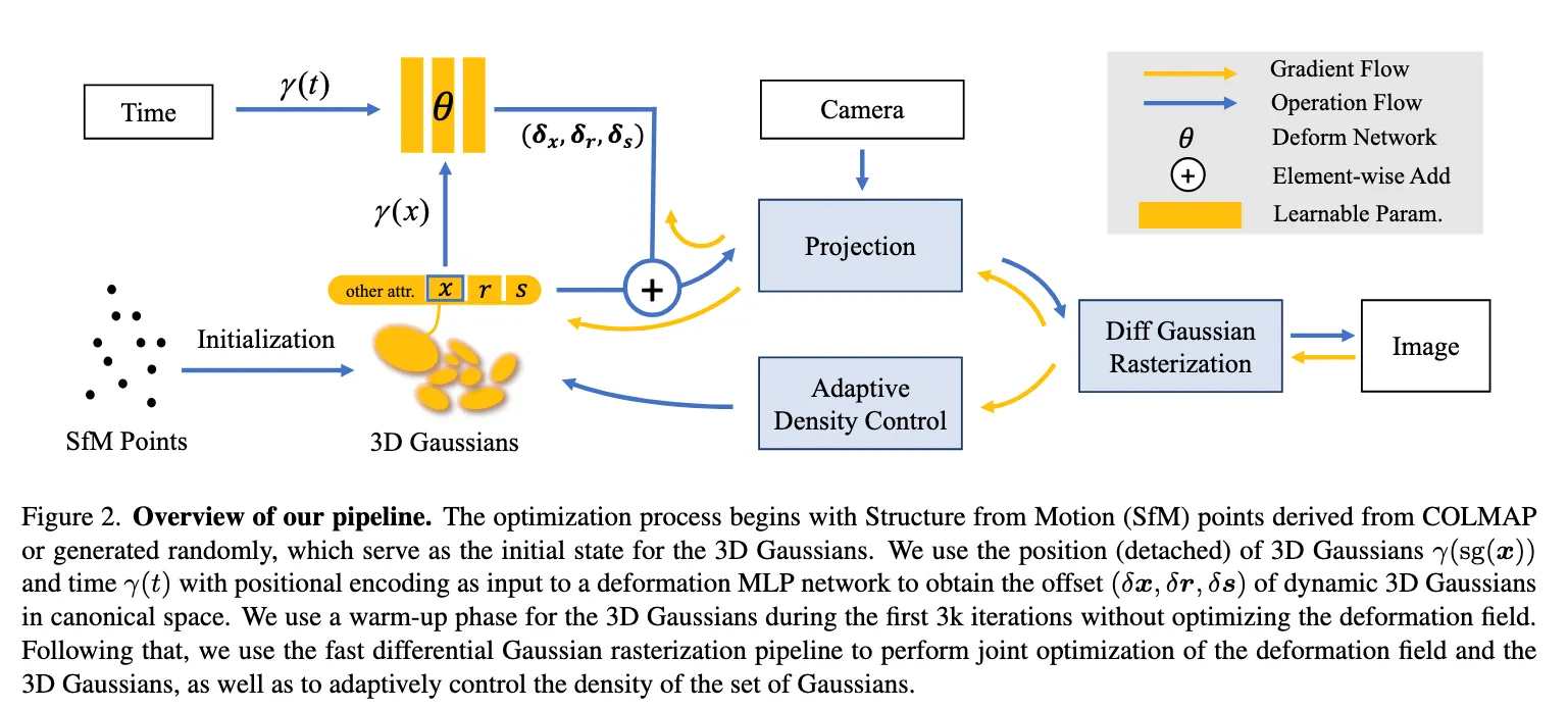
3. Deformable 3D Gaussians (Deformable-GS) [3]

3.1. Canonical space plus a deformation field

Deformable-GS keeps 3D Gaussians $(\mu,\Sigma,\alpha)$ in a time-independent canonical frame and learns a deformation MLP $F_\theta$ that maps position and time with positional encodings to offsets for position $\delta \mathbf{x}$, rotation $\delta r$ as a quaternion, and scale $\delta s$. At time $t$:

where $\gamma(\cdot)$ is a positional encoding and $\oplus$ denotes quaternion composition. The updated Gaussian at $t$ is rendered by the standard 3DGS pipeline using the projected 2D covariance $\Sigma'$.

Why canonicalization helps. By decoupling geometry from motion, we avoid storing time-varying primitives and can tap into the mature 3DGS stack. This is especially attractive for monocular dynamics where multi-view redundancy is scarce.

3.2. Annealing Smoothing Training (AST)

Monocular captures often exhibit early spatial jitter because motion is under-constrained or late over-smoothing that loses detail. AST addresses both with a time-varying smoothness prior on the deformation field.

This schedule improves temporal smoothness and structural consistency on real-world monocular scenes while avoiding late-stage blur.

3.3. Training regimen and pitfalls

• Warm-up. Train only the Gaussians for about 3k iterations to stabilize positions and shapes.
• Joint phase. Then train Gaussians plus deformation for the remaining about 37k iterations, at 800×800 on a high-end GPU.
• Positional encoding. Apply PE to both position and time to sharpen details.
• Camera poses. Inaccurate poses are detrimental for explicit point-based rendering and can derail convergence. Refine with COLMAP or add small learnable pose refinements with priors.
• Few-shot risk. Narrow baselines or very few views can overfit even for vanilla 3DGS. Use data augmentation, stronger AST early, and viewpoint-balanced batches.
• Dataset splits. In some cases, swapped train and test with sufficient views around 100 exhibits much improved generalization.

3.4. Losses

• Photometric. $\mathcal{L}=(1 - \lambda)\mathcal{L}_1 + \lambda_\text{ssim} \mathcal{L}_\text{D-SSIM}$.
• Scale and opacity priors. Small $L_2$ or log-space regularizers to avoid degenerate growth and optional opacity entropy to keep footprints crisp.

4. 4DGS vs. Deformable-GS: What to use when

Both support monocular. 4DGS demonstrates single-view-per-time results similar to D-NeRF setups. Deformable-GS explicitly targets monocular dynamics and introduces AST.

Expressivity

• 4DGS. By letting primitives rotate and tilt in $(x,y,z,t)$, 4DGS naturally aligns with motion manifolds. Intrinsic dynamics can emerge without explicit motion supervision.
• Deformable-GS. Factorizes geometry and motion. Flexible and modular, but highly non-rigid scenes may demand a wider deformation head and stronger priors.

Appearance modeling

• 4DGS. SH × Fourier models view-dependent appearance that evolves in time, useful when both motion and appearance change such as specularities or lighting.
• Deformable-GS. Often retains standard 3D SH and explains temporal changes mainly via motion. This is simpler with fewer coefficients.

Speed and scalability

• Both inherit real-time rendering from 3DGS.
• 4DGS. Spacetime locality keeps long-clip rendering efficient. Add marginal gating $\pi_i(t)$ to cull inactive primitives.
• Deformable-GS. Reuses a familiar stack and can have fewer parameters than storing per-time primitives.

Data and supervision

• 4DGS. Benefits from multi-view, but also works on monocular. Can leverage sparse LiDAR for depth supervision and often needs background initialization for far geometry.
• Deformable-GS. Designed for monocular. Most sensitive to pose accuracy. Use AST and modest PE to stabilize.

Failure modes and mitigations

4DGS:

• Missed distant background leads to artifacts. Add a frozen spherical cloud.
• Over-reconstruction in spacetime. Cap time modes, gate by $\pi_i(t)$, and stop growing the temporal basis early.

Deformable-GS:

• Pose noise harms convergence. Refine or jointly optimize with priors.
• Few-shot overfit. Use data augmentation plus stronger early AST and more diverse view sampling.

5. Repro Checklist for Monocular Setups

1. Poses. Run COLMAP with thorough matching. If needed, enable bundle adjustment refinement. For Deformable-GS, consider small learnable pose tweaks with strong priors.
2. Initialization.
   • 4DGS: Seed a spherical background and freeze early.
   • Deformable-GS: Initialize canonical Gaussians via a 3DGS warm-up of about 3k iterations.
3. Time sampling. Uniform or per-frame proportional. Use small $\delta$ strides to form AST triplets.
4. Losses. L1 plus SSIM photometric, AST velocity and acceleration, small scale and opacity priors. Optional sparse depth if available.
5. Schedules.
   • 4DGS: About 30k iterations, turn densification off halfway, temporal marginal gate $\pi_i(t)<0.05$.
   • Deformable-GS: 40k total at 800×800. Positional encoding on $x$ and $t$.
6. Diagnostics. Track LPIPS and SSIM and a short temporal flicker metric such as frame to frame PSNR or LPIPS. Visualize primitive trajectories $\mu_{x\mid t}$.
7. Failure triage.
   • Flicker suggests increasing early AST.
   • Missed background suggests adding or freezing the background cloud.
   • Pose drift suggests tighter bundle adjustment or enabling pose refinement.

Conclusion

4DGS shows that elevating time to a first-class coordinate yields spacetime primitives that naturally align with motion and support time-evolving appearance in a compact SH × Fourier basis, delivering real-time photo-real video. Deformable-GS keeps a canonical world and learns a motion field with AST regularization, producing robust, high-fidelity reconstructions, especially in monocular captures, while preserving the ergonomic benefits of 3DGS. In practice, your choice reduces to where you place time: inside the primitive (4DGS) or inside the deformation (Deformable-GS).